Golden Age of Television Analysis

import pandas as pd

from siuba import *
from siuba.dply.vector import row_number, n

from plotnine import *

tv_ratings = pd.read_csv(
    "https://raw.githubusercontent.com/rfordatascience/tidytuesday/master/data/2019/2019-01-08/IMDb_Economist_tv_ratings.csv",
    parse_dates = ["date"]
)

Glance at data for a single show

tv_ratings >> filter(_, _.title.str.contains("Buffy"))

	titleId	seasonNumber	title	date	av_rating	share	genres
275	tt0118276	1	Buffy the Vampire Slayer	1997-04-14	7.9629	11.70	Action,Drama,Fantasy
276	tt0118276	2	Buffy the Vampire Slayer	1997-12-31	8.4191	19.41	Action,Drama,Fantasy
277	tt0118276	3	Buffy the Vampire Slayer	1999-01-29	8.6233	17.12	Action,Drama,Fantasy
278	tt0118276	4	Buffy the Vampire Slayer	2000-01-19	8.2205	16.19	Action,Drama,Fantasy
279	tt0118276	5	Buffy the Vampire Slayer	2001-01-12	8.3028	11.99	Action,Drama,Fantasy
280	tt0118276	6	Buffy the Vampire Slayer	2002-01-29	8.1008	8.45	Action,Drama,Fantasy
281	tt0118276	7	Buffy the Vampire Slayer	2003-01-18	8.0460	9.89	Action,Drama,Fantasy

Count season number

(tv_ratings
  >> count(_, _.seasonNumber)
  >> ggplot(aes("seasonNumber", "n"))
   + geom_col()
   + labs(
       title = "Season Number Frequency",
       x = "season number",
       y = "count"
  )
)

<ggplot: (8742457309675)>

Average rating throughout season

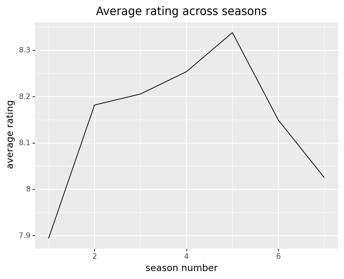
(tv_ratings
  >> filter(_, _.seasonNumber <= 7)
  >> group_by(_, _.seasonNumber)
  >> summarize(_, av_rating = _.av_rating.mean())
  >> ggplot(aes("seasonNumber", "av_rating"))
   + geom_line()
   + labs(
       title = "Average rating across seasons",
       x = "season number",
       y = "average rating"
  )
)

<ggplot: (8742457244853)>

Shows with most variable ratings

Filter down

by_show = (tv_ratings
  >> group_by(_, "title")
  >> summarize(_,
       avg_rating = _.av_rating.mean(),
       sd = _.av_rating.std(),
       seasons = n(_)
     )
  >> arrange(_, -_.avg_rating)
)

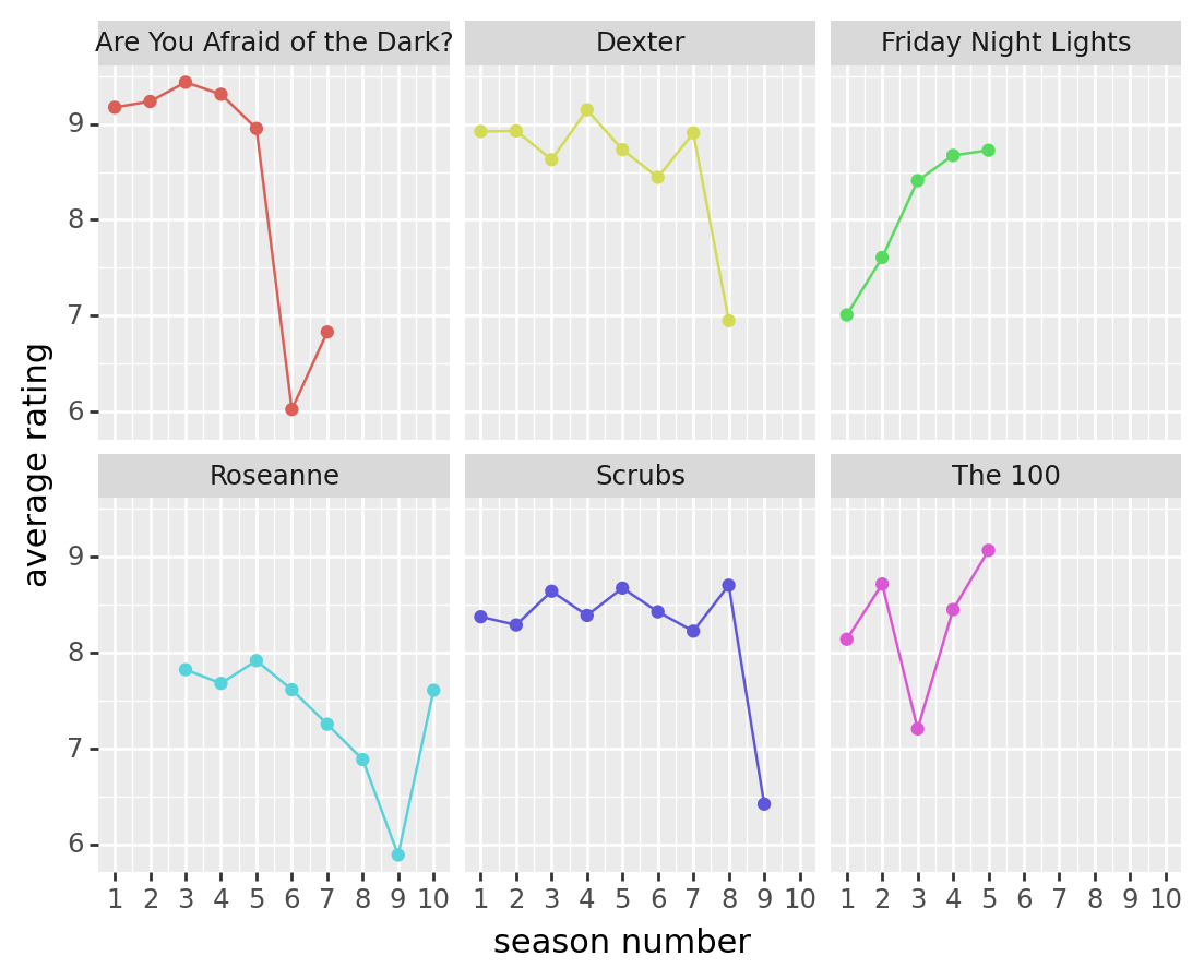
most_variable_shows = (by_show
  >> filter(_, _.seasons >= 5)
  >> arrange(_, -_.sd)
  >> head(_, 6)
)

most_variable_shows

	title	avg_rating	sd	seasons
49	Are You Afraid of the Dark?	8.422971	1.390834	7
263	Friday Night Lights	8.085020	0.749403	5
650	The 100	8.314140	0.708071	5
582	Scrubs	8.236744	0.702544	9
195	Dexter	8.582400	0.694169	8
562	Roseanne	7.332537	0.670299	8

Plot show ratings

(tv_ratings
  >> inner_join(_, most_variable_shows, "title")
  >> ggplot(aes("seasonNumber", "av_rating", color = "title"))
   + geom_line()
   + geom_point()
   + scale_x_continuous(breaks = range(11))
   + facet_wrap("~ title")
   + theme(legend_position = "none")
   + labs(
       x = "season number",
       y = "average rating"
  )
)

<ggplot: (8742455023836)>