from siuba import (
    _,
    inner_join, left_join, full_join, right_join,
    semi_join, anti_join
)

lhs = pd.DataFrame({'id': [1,2,3], 'val': ['lhs.1', 'lhs.2', 'lhs.3']})
rhs = pd.DataFrame({'id': [1,2,4], 'val': ['rhs.1', 'rhs.2', 'rhs.3']})Join tables
Joins allow you to combine data from two tables, using two steps:
- determining matches in values between a set of specified columns.
- merging columns from matching rows into a new table.
The number of ways joins can be used is surprisingly deep, and provides an important foundation for most data analyses!
lhs| id | val | |
|---|---|---|
| 0 | 1 | lhs.1 |
| 1 | 2 | lhs.2 |
| 2 | 3 | lhs.3 |
rhs| id | val | |
|---|---|---|
| 0 | 1 | rhs.1 |
| 1 | 2 | rhs.2 |
| 2 | 4 | rhs.3 |
Note
The format of graphs and the structure of examples takes heavy inspiration from R for Data Science.
Syntax
Like other siuba verbs, joins can be used in two ways: by directly passing both data as arguments, or by piping.
# directly passing data
inner_join(lhs, rhs, on="id")

# piping
lhs >> inner_join(_, rhs, on="id")| id | val_x | val_y | |
|---|---|---|---|
| 0 | 1 | lhs.1 | rhs.1 |
| 1 | 2 | lhs.2 | rhs.2 |
Note that when used in a pipe, the first argument to the join must be _, to represent the data.
How joins work
This page will use graphs to illustrate how joins work. They show the values being joined on for the left-hand side on the rows, and those for the right-hand side on the columns.
For example, consider the inner join from the last section:
inner_join(lhs, rhs, on="id")| id | val_x | val_y | |
|---|---|---|---|
| 0 | 1 | lhs.1 | rhs.1 |
| 1 | 2 | lhs.2 | rhs.2 |
Here is a graph for this inner join:
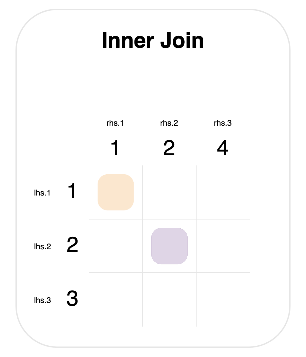
Notice that 1, 2, 3 come from the lhs.id column, and 1, 2, 4 from rhs.id.
There are two steps to any join:
- Determine matches. The colored squares mark new rows that will be created. These are determined by looking at every pair of values from the left- and right-hand sides, and checking whether they’re equal. This means that there are 9 checks in total (one for each square in the grid).
- Merge rows. For each match, a row is created that has columns from both tables.
The next two sections on this page discuss different types of joins:
- Mutating joins: what should happen if a row or column doesn’t have any matches?
- Filtering joins: using matching rules without merging to filter the left-hand table.
The remaining four sections discuss important situations related to matching: duplicates, missing values, using multiple columns, and expressions.
Mutating joins
Up to this point we’ve looked at an inner join. We’ll call this a mutating join, because it puts the columns from both tables into the final result. In this section, we’ll look at two more important joins: left join and full join.
The diagram below shows these three mutating joins.
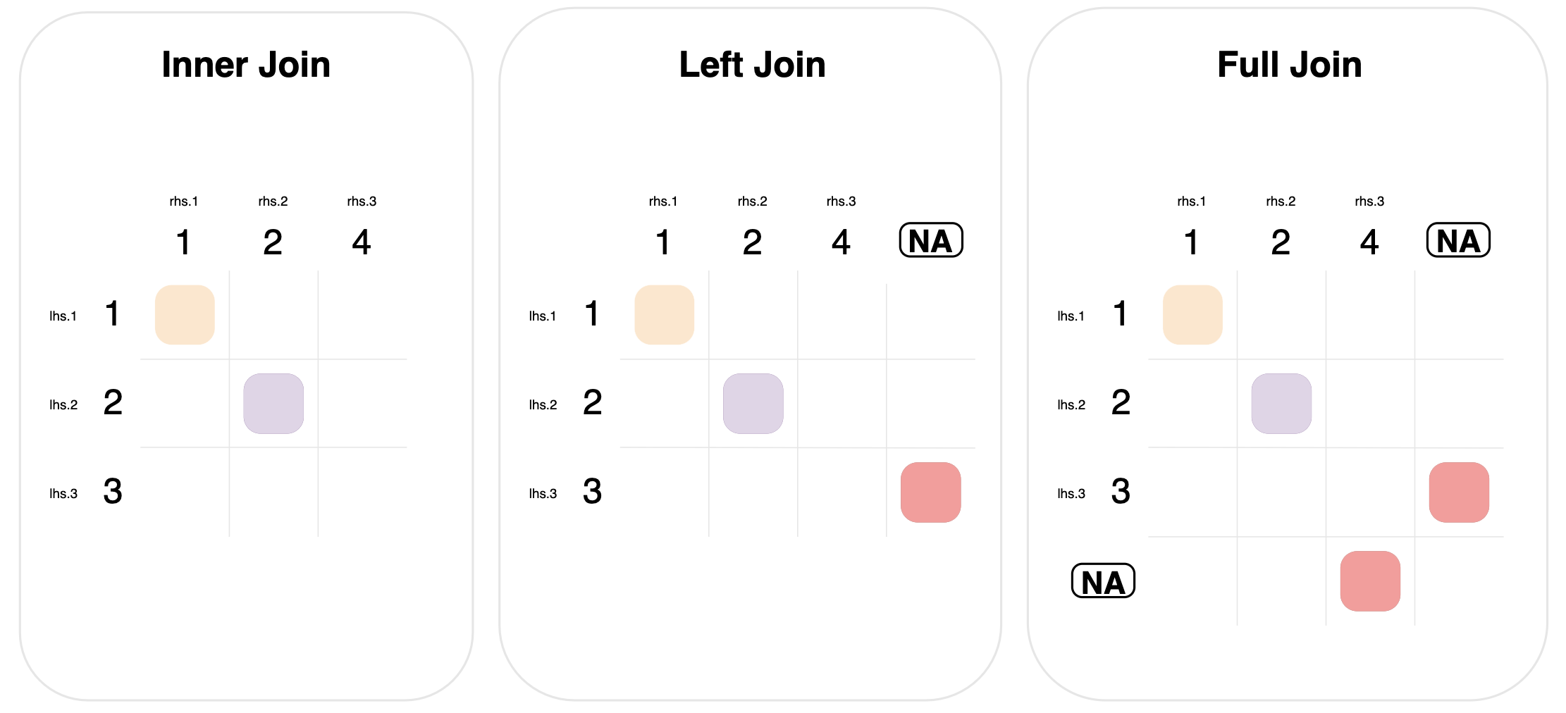
Left and full joins define a new matching rule for rows of data that don’t have any matches:
Left join. Include rows from the left-hand table that didn’t have any matches. This is done by matching left-hand rows with no matches, to a “dummy” right-hand row of all missing values. This is signified in the graph by the circled NA column.
Full join: Similar to left join, but extended to include unmatched rows from both tables. Notice that the graph for full join has two “dummy circled NA” entries, one to match rows, and one to match columns.
Inner join
inner_join(lhs, rhs, on="id")| id | val_x | val_y | |
|---|---|---|---|
| 0 | 1 | lhs.1 | rhs.1 |
| 1 | 2 | lhs.2 | rhs.2 |
Outer joins
left_join(lhs, rhs, on="id")| id | val_x | val_y | |
|---|---|---|---|
| 0 | 1 | lhs.1 | rhs.1 |
| 1 | 2 | lhs.2 | rhs.2 |
| 2 | 3 | lhs.3 | NaN |
full_join(lhs, rhs, on="id")| id | val_x | val_y | |
|---|---|---|---|
| 0 | 1 | lhs.1 | rhs.1 |
| 1 | 2 | lhs.2 | rhs.2 |
| 2 | 3 | lhs.3 | NaN |
| 3 | 4 | NaN | rhs.3 |
Filtering joins
Filtering joins use some of the same logic to determine matches as a join, but only to filter (remove) rows from the left-hand table.
We’ll use the data from the previous section to look at filtering joins.
lhs| id | val | |
|---|---|---|
| 0 | 1 | lhs.1 |
| 1 | 2 | lhs.2 |
| 2 | 3 | lhs.3 |
rhs| id | val | |
|---|---|---|
| 0 | 1 | rhs.1 |
| 1 | 2 | rhs.2 |
| 2 | 4 | rhs.3 |
Use semi_join() to keep rows in the left-hand table that would have a match:
semi_join(lhs, rhs, on="id")| id | val | |
|---|---|---|
| 0 | 1 | lhs.1 |
| 1 | 2 | lhs.2 |
Use anti_join() to keep the rows that a semi_join() would drop—the rows with no matches:
anti_join(lhs, rhs, on="id")| id | val | |
|---|---|---|
| 2 | 3 | lhs.3 |
Duplicate matches
Mutating joins create a new row for each match between value pairs. This means that a join can duplicate rows from the left- or right-hand data.
For example, consider the situation where the left- and right-hand data both have the value 2 multiple times in the columns they’re joining on.

This is shown in the graph above—for an inner join, where both tables contain the value 2 twice. In this case, it results in 4 matches, which will each produce a row in the final result.
Here is the code corresponding to the graph above.
import pandas as pd
lhs_dupes = pd.DataFrame({
    "id": [1, 2, 2, 3],
    "val": ["lhs.1", "lhs.2", "lhs.3", "lhs.4"]
})

rhs_dupes = pd.DataFrame({
    "id": [1, 2, 2, 4],
    "val": ["rhs.1", "rhs.2", "rhs.3", "rhs.4"]
})lhs_dupes| id | val | |
|---|---|---|
| 0 | 1 | lhs.1 |
| 1 | 2 | lhs.2 |
| 2 | 2 | lhs.3 |
| 3 | 3 | lhs.4 |
rhs_dupes| id | val | |
|---|---|---|
| 0 | 1 | rhs.1 |
| 1 | 2 | rhs.2 |
| 2 | 2 | rhs.3 |
| 3 | 4 | rhs.4 |
inner_join(lhs_dupes, rhs_dupes, on="id")| id | val_x | val_y | |
|---|---|---|---|
| 0 | 1 | lhs.1 | rhs.1 |
| 1 | 2 | lhs.2 | rhs.2 |
| 2 | 2 | lhs.2 | rhs.3 |
| 3 | 2 | lhs.3 | rhs.2 |
| 4 | 2 | lhs.3 | rhs.3 |
NA handling
By default, missing values are matched to each other in joins.
This is shown in the left join below, where each table has a single NA value.
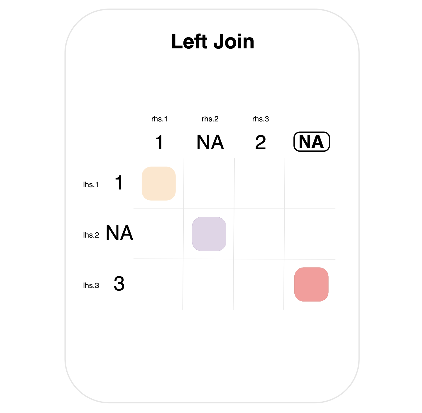
Note the purple mark indicating a match between the NA values. Importantly, literal NA values here are different from the circled dummy NA (top right), which indicates the special matching rule for left joins.
Here is the code for the example:
import pandas as pd
lhs_na = pd.DataFrame({"id": [1, pd.NA, 3], 'val': ['lhs.1', 'lhs.2', 'lhs.3']})
rhs_na = pd.DataFrame({"id": [1, pd.NA, 2], 'val': ['rhs.1', 'rhs.2', 'rhs.3']})
left_join(lhs_na, rhs_na, on="id")| id | val_x | val_y | |
|---|---|---|---|
| 0 | 1 | lhs.1 | rhs.1 |
| 1 | <NA> | lhs.2 | rhs.2 |
| 2 | 3 | lhs.3 | NaN |
Match on multiple columns
Joins can be performed by comparing multiple pairs of columns to each other— such as the source and id columns in the data below.
lhs_multi = pd.DataFrame({
    "source": ["a", "a", "b"],
    "id": [1, 2, 1],
    "val": ["lhs.1", "lhs.2", "lhs.3"]
})

rhs_multi = pd.DataFrame({
    "source": ["a", "b", "c"],
    "id": [1, 1, 1],
    "val": ["rhs.1", "rhs.2", "rhs.3"]
})lhs_multi| source | id | val | |
|---|---|---|---|
| 0 | a | 1 | lhs.1 |
| 1 | a | 2 | lhs.2 |
| 2 | b | 1 | lhs.3 |
rhs_multi| source | id | val | |
|---|---|---|---|
| 0 | a | 1 | rhs.1 |
| 1 | b | 1 | rhs.2 |
| 2 | c | 1 | rhs.3 |
In this case, a match happens when source matches AND id matches—as shown by the composite values (source, id) in the graph below.
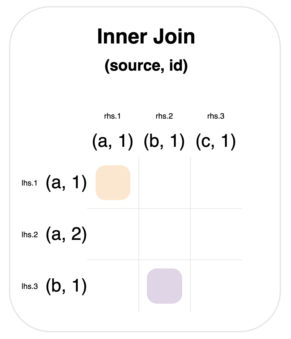
Using a list of columns
Use the on= argument with a list of columns, in order to join on multiple columns.
inner_join(lhs_multi, rhs_multi, on=["source", "id"])| source | id | val_x | val_y | |
|---|---|---|---|---|
| 0 | a | 1 | lhs.1 | rhs.1 |
| 1 | b | 1 | lhs.3 | rhs.2 |
Using a dictionary of columns
Use the on= argument with a dictionary to join pairs of columns with different names.
from siuba import rename

rhs_multi2 = rename(rhs_multi, some_source = "source")

inner_join(lhs_multi, rhs_multi2, {"source": "some_source", "id": "id"})| source | id | val_x | some_source | val_y | |
|---|---|---|---|---|---|
| 0 | a | 1 | lhs.1 | a | rhs.1 |
| 1 | b | 1 | lhs.3 | b | rhs.2 |
Match on expressions
Some siuba backends—like those that execute SQL—can join by expressions for determining matches.
For example, the graph below shows an inner join, where a match occurs when the left-hand value is less than or equal to the right-hand value.
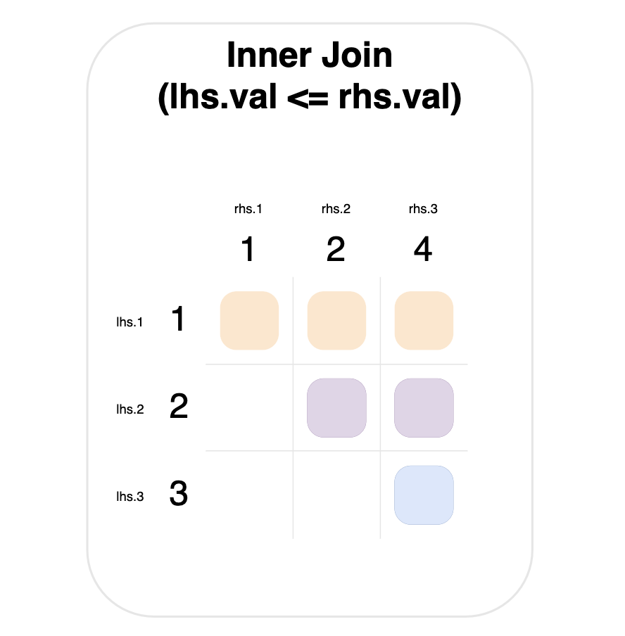
Notice that the value 1 on the left-hand side matches everything on the right-hand side (top row).
SQL backend sql_on argument.
Here is a full example, using sqlite:
from sqlalchemy import create_engine
from siuba.sql import LazyTbl

engine = create_engine("sqlite:///:memory:")

lhs = pd.DataFrame({'id': [1,2,3], 'val': ['lhs.1', 'lhs.2', 'lhs.3']})
rhs = pd.DataFrame({'id': [1,2,4], 'val': ['rhs.1', 'rhs.2', 'rhs.3']})

lhs.to_sql("lhs", engine, index=False)
rhs.to_sql("rhs", engine, index=False)

tbl_sql_lhs = LazyTbl(engine, "lhs")
tbl_sql_rhs = LazyTbl(engine, "rhs")

inner_join(
    tbl_sql_lhs,
    tbl_sql_rhs,
    sql_on = lambda lhs, rhs: lhs.val <= rhs.val
)
# Source: lazy query # DB Conn: Engine(sqlite:///:memory:) # Preview:
| id_x | val_x | val_y | id_y | |
|---|---|---|---|---|
| 0 | 1 | lhs.1 | rhs.1 | 1 |
| 1 | 1 | lhs.1 | rhs.2 | 2 |
| 2 | 1 | lhs.1 | rhs.3 | 4 |
| 3 | 2 | lhs.2 | rhs.1 | 1 |
| 4 | 2 | lhs.2 | rhs.2 | 2 |
# .. may have more rows
Note that the function passed to sql_on takes sqlalchemy columns for the left- and right-hand sides, so currently limited to what can be done in sqlalchemy.